Laplace’s sun rise problem (rule of succession), some simple thoughts

Today I happened to visit the wiki page of Pierre-Simon Laplace. And saw the sun rise problem. I only have a quite vague memory of it so I decided to read through. The problem is quite simple: you have seen the sun rise for the past $N$ days, what is the probability that the sun will rise tomorrow? The extra settings are basically to assume the probability of the sun rise is $p$ , which is uniformly distributed in [0,1]. The likelihood of seeing $X$ days of sun rise is simply $p^X(1-p)^{(N-X)}$ . If you have seen sun rising for all the days, then $X=N$ . After that the posterior is the likelihood divided by a normalization factor (check out here for how the integral is computed):

$pdf(p) = \frac{(N+1)!}{X!(N-X)!}p^X(1-p)^{(N-X)}$

Using law of total probability, which means $P(sun rise) = \sum{P(sun rise|p)*P(p)}$ (And of course in this case there should be integral instead of summation), one get $P(sunrise) = \frac{X+1}{N+2}$ .

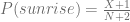
That means, for someone like me, 28.5 years (7553 days) of seeing or knowing (yes, it rains) the sun rises, the probability of sun not rising tomorrow is 0.014%. Which is actually not as small as I thought….

Now, here are the two questions I want to address.

Are we using uniform prior here? Or we are using beta distribution as prior? Different sources are different.
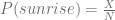
Why not $P(sunrise) = \frac{X}{N}$

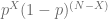
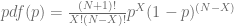
The first one confused me for a while today. From most of the places I read about this problem, people mention they assume a uniform prior for $p$ , but is that the whole story?

Of course not. You can also use beta distribution, and actually they are equivalent. Using uniform prior from the beginning and compute the posterior after N days is equivalent to using a beta distribution (start with $\alpha=1$ and $\beta=1$ at day 1, which is uniform distribution), updating the posterior each day and using yesterday’s posterior as today’s prior. How do we know they are equivalent? Well you can look at the posterior pdf again and realize updating it with another success is just adding $X$ by 1. It is the natural convenience of the conjugated prior. (It is also the first time I feel good about conjugated prior-I think people emphasize too much on “being convenient”, why we need convenience when we are looking for answers?)

The second one is also quite interesting. The explanation on wiki is like you can get that result if you are “total ignorant of $p$ “. I can’t understand that statement. My answer is actually much simpler. Forget about $p$ being a probability, and suppose we have a machine with a parameter $p$ , which we don’t know. Our hypothesis of $p$ ‘s value is uniformly distributed in [0,1]. Given that we have observed X of successes of N-X of failures, what is the most probable value of p?

No doubt, $\frac{X}{N}$

Why? Because it is not computing the mean of posterior, rather it is computing the mode (or, maximize a posteriori, MAP, the maxima of the posterior distribution).When the distribution is skewed, the expectation and mode will be different. (Not the case for ridge regression, which is actually computed using MAP)

There are a lot of articles talking about MAP, pros and cons, attacks and defense. But all in all, I think it is much convenient to use for both value and variance estimation 😀