
The go games between Lee Sedol and AlphaGo have aroused a huge wave of discussion on AI and machine learning. This article is actually from a joke-like idea that I made several days ago that I would write an AI for paper, scissors, rock. The reason such AI is almost meaningless is that each match is independent from each other. Therefore the algorithm can only utilize information if the player does have a strategy, explicitly or implicitly (It is quite possible, and I will write one this month). Anyway, then I decide to do a simpler experiment first to answer a question:
How complex a network need to be to simulate paper, scissors, rock?
The problem is, paper, scissor, rock is not an easy numerical problem. There are two major differences: 1. In basic math, there is always such a rule: A->B and B->C lead to A->C, which is apparently not the case for this game; 2. All the features (the appearance of each choice, dummy variable) have the strict correlation of zero with the outcome (you have equal chances of winning, losing or getting tie if you make a paper).
The all possible input data is quite small:
allpossiblemoves = np.array([
['p','p',0],
['p','r',1],
['s','p',1],
['r','s',1],
['r','r',0],
['s','s',0],
['r','p',-1],
['s','r',-1],
['p','s',-1]
])
First of all, can a multi-class logistic regression make it happen? I used the logistic regression from sklearn to do the learning. And the confusion matrix is like this:
[[3 0 0]
 [3 0 0]
 [3 0 0]]
Logistic regression failed. Then I start to use the neural network. To make the visulization easier, I developed this function:
def nnvis(W,feature_names="",threshold=0.5):
        #W is the dictionary of all the weights, keys start from 1
        #The dimension of W is d1 by d2, so np.dot(X,W[1]) should work (with or without intercept)
	import networkx as nx
	G = nx.Graph()
	pos={}
	layer = len(W.keys())
	actdim = []
	outdim = W[layer].shape[1]
	for l in range(layer):
		actdim.append(W[l+1].shape[0])

	for l in range(layer):
		for j in range(actdim[l]):
			G.add_node((l,j))
			pos[(l,j)] = (j,l)

	for j in range(outdim):
		G.add_node((layer,j))
		pos[(layer,j)] = (j,layer)

	edge_labels = {}

	for l in range(layer):
		Wc = W[l+1]
		maxw = -1e5
		minw = 1e5
		for i in range(actdim[l]):
			for j in range(W[l+1].shape[1]):
				G.add_weighted_edges_from([((l,i),(l+1,j),trunc(Wc[i,j]))])
				if(trunc(Wc[i,j])>maxw):
					maxw = trunc(Wc[i,j])
					maxwpos = ((l,i),(l+1,j))
				if(trunc(Wc[i,j])<minw):
                                        minw = trunc(Wc[i,j])
                                        minwpos = ((l,i),(l+1,j))
                 edge_labels.update({maxwpos:maxw,minwpos:minw})

        weights = [d['weight'] for (u,v,d) in G.edges(data=True)]
        edge_color = [i if abs(i)>threshold else 0 for i in weights]
	labels = {}
	for j in range(min(actdim[0],len(feature_names))):
		labels[(0,j)]="\n"+feature_names[j]

	props = dict(facecolor='wheat',alpha=0.5)
	nx.draw(G,pos=pos,edge_color = edge_color,
			width = [abs(i) for i in edge_color],
			edge_cmap = plt.get_cmap('seismic'),
			labels = labels,
			font_size=20,font_weight=10)
	edge_labels = nx.draw_networkx_edge_labels(G,pos=pos,alpha=0.6,
                       edge_labels=edge_labels,
                       bbox=props)
	plt.show()
And for a network of 7-2-3, the network is like this (blue is negative, red is positive and linewidth is proportional to the absolute value):
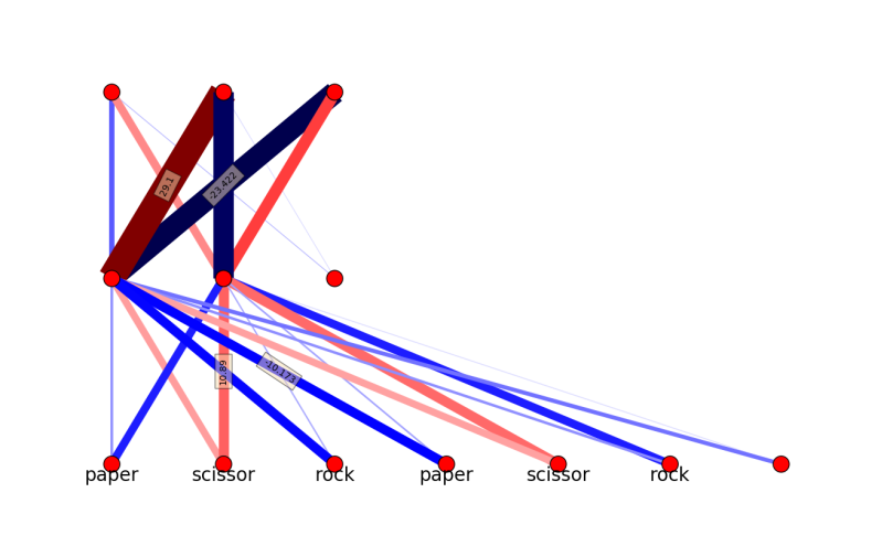
No matter how many times I tried, the training accuracy is never 1.0. Then I increase the inner nodes to be 3:
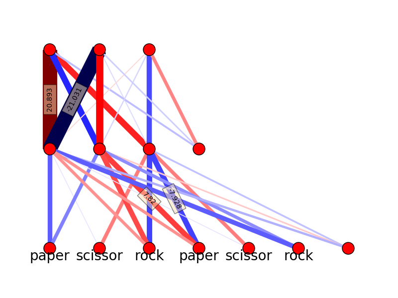
I still need to run several times to find the solution with accuracy 1.0, that may indicate that the actual number of solutions is quite small. The outputs of the inner nodes for all the possible combinations listed in this article are:
['p','p',0],[ 3.65102518e-03 9.92082441e-01 2.27972412e-05]
['p','r',1],[ 5.29280637e-08 4.44827194e-04 4.44386986e-02]
['s','p',1],[ 4.82426841e-01 9.99949399e-01 5.78623844e-03]
['r','s',1],[ 4.82469321e-01 9.99949334e-01 5.82915306e-03]
['r','r',0],[ 3.66621886e-03 9.92074408e-01 2.29786956e-05]
['s','s',0],[ 3.39925446e-03 9.17122885e-01 9.99669995e-01]
['r','p',-1],[ 9.96090081e-01 9.99999972e-01 1.12648332e-08]
['s','r',-1],[ 1.34628358e-05 6.55821913e-02 9.22312531e-01]
['p','s',-1],[ 1.34091200e-05 6.55663650e-02 9.22277006e-01]

In this network, the inner nodes have very distinguished functions. Node 1 is only activated by 'r,p,-1','s,p,1','r,s,1', while the node 2 is activated by 'p,p,0','s,p,1','r,s,1','r,r,0','s,s,0','r,p,-1' and node 3 is activated by 's,s,0','s,r,-1' and 'p,s,-1'

The activation list:
['p','p',0],2
['p','r',1],
['s','p',1],1*,2
['r','s',1],1*,2
['r','r',0],2
['s','s',0],2,3
['r','p',-1],1,2
['s','r',-1],3
['p','s',-1],3
The intepretation is still hard due to the intrinic complexity of the network, but it is still possible to see something from the list. First, node 2 is mainly for tie. Second, node 3 is for ‘s’ related, and by itself it is only for losing. The winning scheme is quite complicated and hard to intepret.
Actually, if nodes can only provide an “on-or-off” signal, two inner nodes seem to be enough (2^2=4>3) and three inner nodes (2^3=8>>3) seem to be redundant. It is interesting to see if there are any further constraints.
The whole code:
#paper scissor rock

#This first network, logistic regression

from sklearn.linear_model import LogisticRegression as LR
import numpy as np
from sklearn.metrics import confusion_matrix as cfmat
from Ann import *
import matplotlib.pyplot as plt

def trunc(d, num=3):
	before_dec, after_dec = str(float(d)).split('.')
	return float('.'.join((before_dec, after_dec[0:num])))


def nnvis(W,feature_names="",threshold=0.5):
	import networkx as nx
	G = nx.Graph()
	pos={}
	layer = len(W.keys())
	actdim = []
	outdim = W[layer].shape[1]
	for l in range(layer):
		actdim.append(W[l+1].shape[0])

	for l in range(layer):
		for j in range(actdim[l]):
			G.add_node((l,j))
			pos[(l,j)] = (j,l)

	for j in range(outdim):
		G.add_node((layer,j))
		pos[(layer,j)] = (j,layer)

	edge_labels = {}

	for l in range(layer):
		Wc = W[l+1]
		maxw = -1e5
		minw = 1e5
		for i in range(actdim[l]):
			for j in range(W[l+1].shape[1]):
				G.add_weighted_edges_from([((l,i),(l+1,j),trunc(Wc[i,j]))])
				if(trunc(Wc[i,j])>maxw):
					maxw = trunc(Wc[i,j])
					maxwpos = ((l,i),(l+1,j))
				if(trunc(Wc[i,j])<minw):
                                        minw = trunc(Wc[i,j])
                                        minwpos = ((l,i),(l+1,j))
	          edge_labels.update({maxwpos:maxw,minwpos:minw})
        weights = [d['weight'] for (u,v,d) in G.edges(data=True)]
        edge_color = [i if abs(i)>threshold else 0 for i in weights]

	labels = {}
	for j in range(min(actdim[0],len(feature_names))):
		labels[(0,j)]="\n"+feature_names[j]

	props = dict(facecolor='wheat',alpha=0.5)
	nx.draw(G,pos=pos,edge_color = edge_color,
			width = [abs(i) for i in edge_color],
			edge_cmap = plt.get_cmap('seismic'),
			labels = labels,
			font_size=20,font_weight=10)
	edge_labels = nx.draw_networkx_edge_labels(G,pos=pos,alpha=0.6,edge_labels=edge_labels,bbox=props)
	plt.show()

#Now data for input
possiblemoves = np.array([
	['p','p',0],
	['p','r',1],
	['s','p',1],
	['r','s',1],
	['r','r',0],
	['s','s',0]
	])

allpossiblemoves = np.array([
	['p','p',0],
	['p','r',1],
	['s','p',1],
	['r','s',1],
	['r','r',0],
	['s','s',0],
	['r','p',-1],
	['s','r',-1],
	['p','s',-1]
	])

import sklearn
movetable = {'p':0,'s':1,'r':2}

respall = allpossiblemoves[:,-1].astype(int)
print respall
featureall = np.zeros([allpossiblemoves.shape[0],(allpossiblemoves.shape[1]-1)*3])
for i in xrange(featureall.shape[0]):
	index_to_fill1 = movetable[allpossiblemoves[i,0]]
	featureall[i,index_to_fill1]=1
	index_to_fill2 = movetable[allpossiblemoves[i,1]]
	featureall[i,3+index_to_fill2]=1

print featureall
LR_model = LR(fit_intercept=True,C=1000,multi_class='multinomial',solver='lbfgs')
LR_model.fit(np.tile(featureall,[100,1]),np.tile(respall,100))
print LR_model.score(featureall,respall)
pred = LR_model.predict(featureall)
print cfmat(respall,pred)
print LR_model.coef_

X=np.tile(featureall,[100,1])
Y=np.tile(respall,100)
Nh=3
W_up,W_low,set_list = mynn(X,Y,Nh=Nh,eps=0.1,eta=0.1,epochs=100)
print W_low
predicted_class = predict_class(featureall,W_low,W_up,set_list)
print "Accuracy: ",compute_accuracy(predicted_class,respall)
print cfmat(respall,predicted_class)
X_ext = np.append(featureall,np.ones([featureall.shape[0],1]),axis=1)
out_low = logistic(np.dot(X_ext,W_low))
out_low_ext = np.append(out_low,np.ones([len(out_low),1]),axis=1)
out_up = softmax_mat(np.dot(out_low_ext,W_up))
print out_low
print out_up

nnvis({1:W_low,2:W_up},feature_names=["paper","scissor","rock"]*2)
